Optimizing Clickhouse: The Tactics That Worked for Us

At LaunchDarkly, we ingest nearly 100 terabytes of observability data from our customers every month.

by Vadim Korolik

LaunchDarkly is an [open source](https://github.com/highlight/highlight) monitoring distribution. We’re building a suite of tools to monitor your web application, and on this blog, we write about the infra challenges we face along the way. If you’re interested in learning more, get started at [app.launchdarkly.com](https://app.launchdarkly.com).

At LaunchDarkly, we ingest nearly 100 terabytes of observability data from our customers every month. A large chunk of the volume goes to our ClickHouse cluster, handling our client’s Logs, Traces, and Session metadata. Not only do we need to gracefully handle the volume and daily spikes in the traffic patterns, but we also need to ensure that the data is ingested in an efficient format that is performant to query.

About a year ago,having onboarded several larger customers, we started hitting scaling issues with our Clickhouse setup that necessitated several phases of improvements to our query and ingest systems.

This post goes through the initial realization and how we tackled it; we went from a largely un-optimized, cpu-heavy clickhouse cluster to a much more efficient, affordable configuration. And more importantly, this yielded a much more “realtime” experience for our customers.

The Incident

Sometime last year, we onboarded a large customer that sent close to 1 billion spans a day, adding another terabyte to our data ingestion. Beyond the total volume, the real problem with this was in the number of small batches of rows inserted into ClickHouse. Our Kafka queue responsible for buffering data started accruing a backlog, and we quickly noticed that the rate of trace insertion into ClickHouse was significantly lower than the number of new records added to Kafka.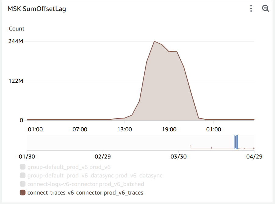

At that time, all we could spot was that ClickHouse had a significant CPU load utilizing all of the available CPU cores of the ClickHouse Cloud Cluster. This seemed to cause the INSERT commands to operate slower in synchronous mode as the cluster created backpressure to reduce the overall CPU load. We also observed “too many parts” errors as ClickHouse was unable to merge the data into fewer parts because of the CPU load. While the hotfix was increasing the CPU allocated the cluster, we quickly had to find a long term solution.

Unlike traditional OTLP SQL, the way that data is written to a ClickHouse table affects query performance. For instance, if data is written in smaller chunks, ClickHouse ends up creating more “parts” (in other words, files) to store it. When querying, ClickHouse has to merge and possibly reorder the results from all relevant parts. Additionally, ClickHouse will asynchronously merge data as it is initially ingested to get it into the right format for long term storage, but this process consumes CPU on background threads that ultimately may decrease performance of concurrent storage. Inserting data with the right configuration helps the merges that ClickHouse has to perform and can speed up how much each merge takes.

Let’s dive into the strategies we used to optimize our ClickHouse cluster and reduce the CPU load.

Reducing Merges - Batch Inserts

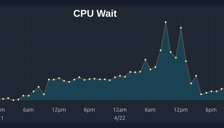
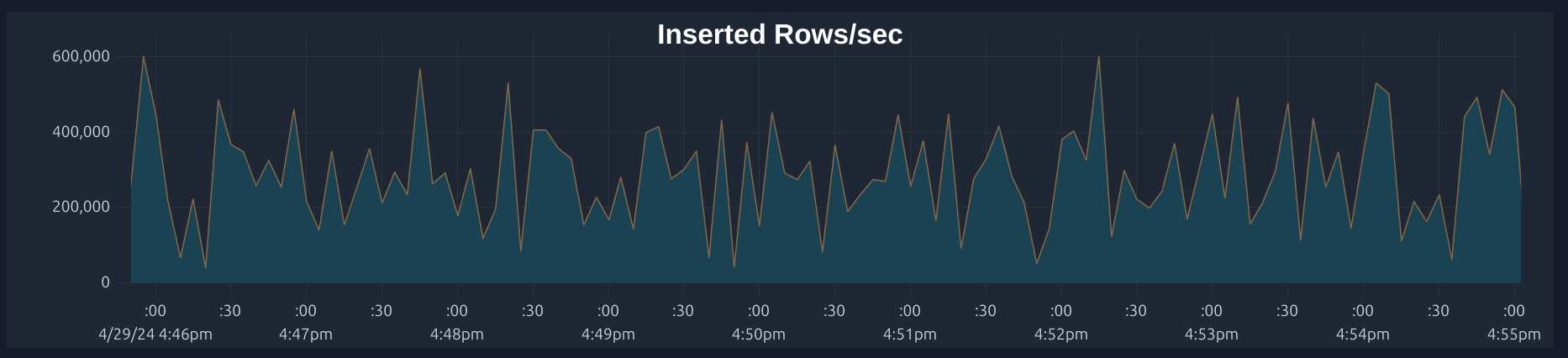
The first step to reducing CPU load on ClickHouse is using larger insert batches. While ClickHouse Cloud offers async inserts to perform individual inserts with the cloud cluster handling batching, we chose to use batch INSERT commands as a way to customize the size of batches on our end. A large batch size was particularly important to our workload as the individual rows were on the order of 100KiB each.

Our first approach used a custom Golang worker that would read messages from Kafka, batch them per our settings, and issue a single INSERT command with many values. Though this worked to ensure inserts were large, inserts were not atomic resulting in duplicate data being inserted during worker reboots.

We opted to use the ClickHouse Kafka Connect Sink that implements batched writes and exactly-once semantics achieved through ClickHouse Keeper.

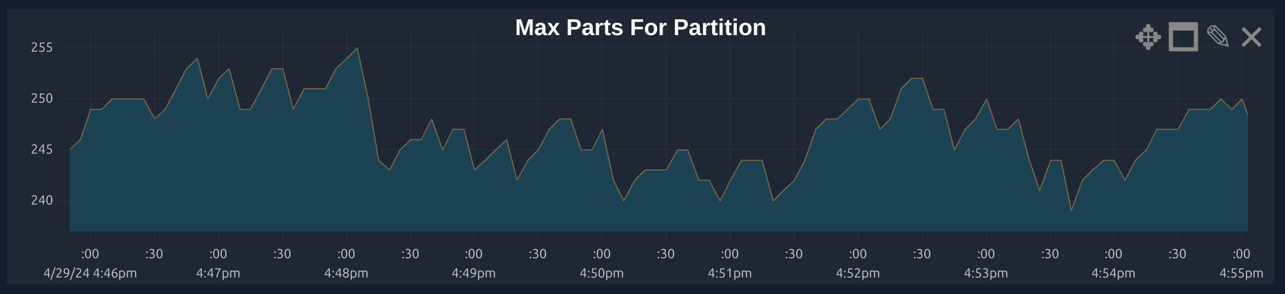
To ensure our changes had the right effect, we monitored the Max Parts graph in ClickHouse for the number of parts waiting to be merged. Read more on how this works from ClickHouse here.

Keeping Data in Wide Parts

CPU Usage during merges can also be incurred by the conversion of parts from compact to wide. When data is inserted compressed, it must be decompressed into the wide format for it to be merged. If inserting large batch sizes (100k+ rows at 10MB+ data), a table level setting that helps is using min_rows_for_wide_part=0, min_bytes_for_wide_part=0 to make sure that ClickHouse will keep inserted data as WIDE to avoid having to convert back and forth between the compact and narrow format, since each conversion incurs a CPU cost.

Optimizing Order By Granularity

If a table is ordered by columns with high granularity, this will result in increased sorting of data when ClickHouse is merging parts. For instance, we found that switching our ORDER BY Timestamp to an ORDER BY toStartOfSecond(Timestamp) reduced the CPU load of merging since everything within the same minute would be grouped into the same part without having to be sorted. The tradeoff occurs with query performance – a granular ORDER BY means that a SELECT will load more parts that must be filtered and sorted, but this is well worth the reduced merging that must happen.

Another common use case for ordering is using a ID. However, adding the ID to the ORDER BY will require all rows to be sorted by a value where each row’s value is unique. A better approach could be to use a truncated version of the ID which would use the first N digits of the value to select a smaller range of rows to sort.

Checking Merge Levels

The performance of merges depends on a number of factors around the type of data and the way that it is inserted. Batch insertion often means that bulk merges may be more efficient. Observing the merge level helps understand how many times data is re-merged within a part. If insertions are large, full part storage is more efficient since the data is already in the right format.

You can also observe all current merges to understand what tables / partitions are causing the most.

select merge_type, merge_algorithm, count()
from clusterAllReplicas(default, system.merges)
where table = 'my_table'
group by 1, 2
order by 3 desc;

If you are inserting in large batches but are still seeing many high-level merges, you may want to adjust the min_bytes_for_full_part_storage setting. For instance,
setting min_bytes_for_full_part_storage=0 will ensure most parts use Full storage which may be more efficient for future large merges as the part_storage_type data format will not have to be converted from Packed to Full.

ALTER TABLE my_table MODIFY SETTING min_bytes_for_full_part_storage = 0;

Avoiding Use of Projections

Projections may be useful to automate switching between multiple views for querying data depending on the primary filter arguments. For example, a table may have a primary key of ORDER BY Timestamp allowing for efficient queries within a time range. At the same time, you may be interested in querying that table by ID. The typical way to do that would be to create a materialized view from the table with a different ORDER BY, and switching the query to select from the materialized view when filtering by ID. Projections offer an automated approach to choosing the source for the select, creating a materialized view for the data but selecting the source automatically. However, with certain queries, the ClickHouse query plan may not select the optimal source view for the data, and it limits your ability to further customize the materialized view. We found using a materialized view and selecting manually as part of our application logic depending on the query pattern to be more reliable.

TTL Optimization / Clearing Old Parts

It’s important to ensure most writes are coming to a few partitions to limit the number of parts that are being merged. Otherwise, ClickHouse will have to merge all parts to keep the data up to date.

A table’s PARTITION BY clause will dictate how data is partitioned. For example, if a table is partitioned by Timestamp, data will be written to different parts based on the timestamp. If you have many concurrent writes with vastly different timestamps, ClickHouse will have to merge many parts as the different writes will land in different active parts. This, in turn, will increase background CPU activity.

In our application (this will depend on your use case), we ensure that most writes are coming to a few partitions, limiting the number of parts that are being merged. We also set a TTL on our tables to clear out old data, which helps with parts remaining active. You can always check how many parts are active by running the following SQL query:

select table, count()
from clusterAllReplicas(default, system.parts)
where active
group by 1
order by 2 desc;

You can see what parts are active across different partitions to understand where writes are landing.

select partition, level, count()
from clusterAllReplicas(default, system.parts)
where active and table = 'my_table'
group by 1, 2, 3
order by 1, 2, 3;

You can also observe all current merges to understand what tables / partitions are causing the most.

select partition, sum(num_parts)
from clusterAllReplicas(default, system.merges)
where table = 'my_table'
group by 1
order by 2 desc;

In our case, we encountered parts that were active and well outside our TTL but still not being deleted. If there is not enough data for a part to be merged, it may not be deleted by the TTL. To the rescue comes a manual command for deleting parts or partitions:

ALTER TABLE my_table
    DROP PARTITION partition_expr;

Conclusion

To conclude, from a largely un-optimized, cpu-heavy clickhouse cluster, we now have a much more efficient, affordable configuration. This experience has also yielded a much more “realtime” experience for our customers. We hope that these strategies can help you optimize your ClickHouse cluster as well. If you have any questions or feedback, feel free to reach out to me on Twitter or LinkedIn.